-
Notifications
You must be signed in to change notification settings - Fork 1
Frederick's Notes
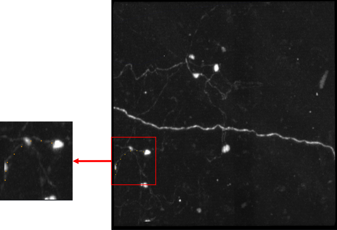
The detailed analysis of the results on non-soma containing images can be found my notebook for Sprint 1. Overall, APP2 has poor performance in the absence of a defined source, such as a soma. The algorithm was designed with a single-source approach in mind, so it is expected that there would be poor performance in images without defined sources. However, we must verify whether or not the shortcomings are a result of image characteristics or an issue with the imaging modality we are working with (Janelia's Mouselight scanners).
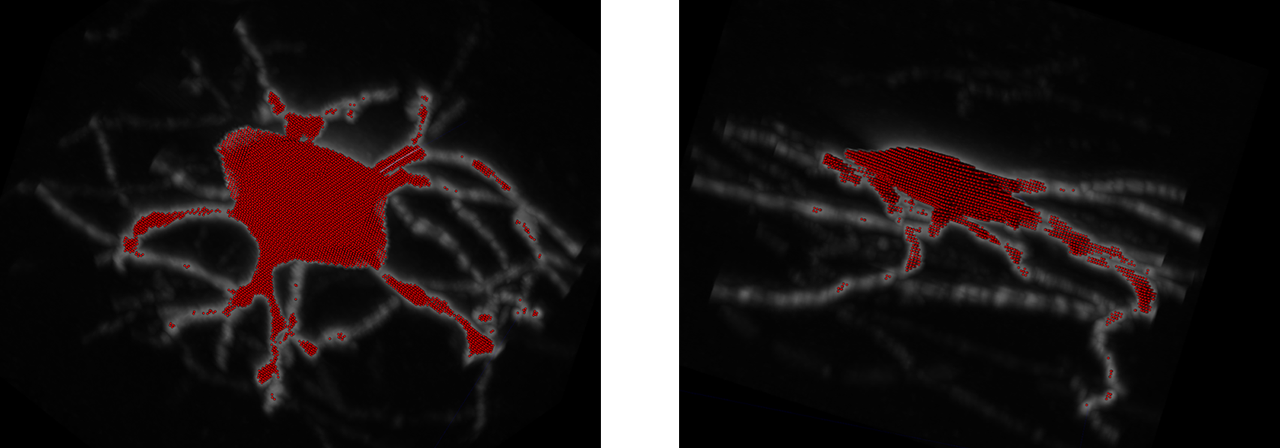
To test this, I ran APP2 on 2 brains where somas were present, pulled from the AWS S3 instance hosting mouselight data. I then ran APP2 locally, and displayed the results in Napari. For a numerical analysis, I performed a 1-way SSD that checked whether or not the ground truth was contained within the trace. Although this relationship seems flipped, our ground truth is a manual trace that is much sparser and more incomplete than what APP2 generates, as the ground truth focuses only on axonal voxels. As such, the 1-way SSD comparing ground truth to the APP2 trace will give an assessment of how accurate APP2 is in reproducing the ground truth, even though it traces beyond the scope of the ground truth.
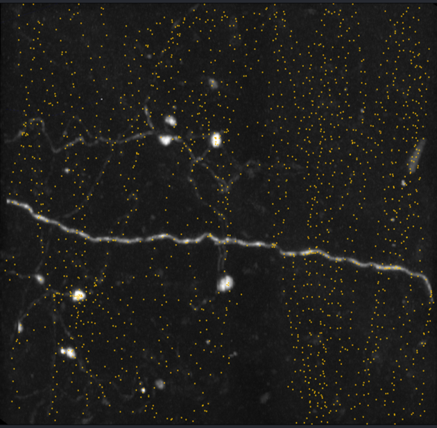
We found that the results for APP2 on soma-containing images were much more promising than the initial tests on benchmarking data. These images were pulled from the AWS S3 instance with a voxel radius of 180 (diameter 360).


For brain1 and brain2, we obtained a 1-way SSD score of 28.47 and 27.15 respectively, which is in the range of the lowest SSD scores from the benchmarking dataset. Additionally, visual fidelity of the trace is quite robust, matching the source image's foreground very closely. This indicates that although APP2 is unusable on mouselight images without somas, it performs adequately on soma-containing mouselight images.
When testing a larger image of voxel radius 500 (diameter 1000), we run into a bottleneck with the napari viewer software where loading the data and subsequently viewing the data is incredibly slow, preventing detailed visual analysis. Additionally, running APP2 took roughly 45 minutes, so I was only able to run the algorithm for brain1:

As we can see, the SSD score is even lower than the smaller image run, at 23.41. However, we can see that APP2 also incorporates other soma-like areas into the trace of the neuron, indicating that the algorithm lacks robustness when discerning between neurons. This will become concerning for future work, as our mouselight data contains multiple neurons in the image, indicating a different approach is necessary.
The plan was to load ground truth (GT) labels for images that ran well, and run DDIV/SSD metrics on them, however I encountered a bug with loading the labels:

I batch tested the APP2 algorithm on the test_gfp benchmarking data. Some of the images ran quite well, although the segmentation is somewhat inaccurate. My plan is to run DDIV and SSD on these images and compare to the ground truth for some data:
test_15-gfp.tif:

test_21-gfp.tif

Other images had some problems, particularly ones with a lot of background noise. Here is an example:
test_11-gfp.tif

For these, I may need to threshold them differently, however the current Vaa3D wrapper that I am using is unable to feed command line parameters to Vaa3D. I will investigate how I can do this in an efficient manner.
File loaded: benchmarking_datasets_test_6-gfp.tif
Settings:
- Default, Background Threshold 10
Result:
Settings:
- Default, Background Threshold -1 (Auto-thresholding)
Result:
NOTE: I had to do this manually through the application. The Python Wrapper does not allow for parameter tuning.
When running APP2, there are actually 2 .swc files that are generated:
- File(1):
brain1_demo_segments.tif_ini.swc - File(2):
brain1_demo_segments.tif_x82_y69_z74_app2.swc
The one that has a coordinate in the filename (such as "_x82_y69_z74_app2") is a sparsely labeled file that looks akin to manually labeled traces. The coordinate in the filename corresponds to the soma, which is the first coordinate of the trace. The only way I was able to tell that this is the true output file is because there is a command prompt line that details the output when the tracing algorithm is ran through the Vaa3D application. I verified the output file is the same when the algorithm is run from the Python Wrapper.
I am unsure what the difference between the two .swc files are. I believe File(1) is an intermediate setup step, hence the "_ini" extension in the title.
The APP2 algorithm also has 2 versions, one with GSDT (GWDT) and one without. The proper algorithm run requires that GSDT be selected, however there is no way to do so in the Python Wrapper. The option is ticked on by default, but if not, it is likely that the algorithm must be run using the application.
Additionally, the skeletonization process is no longer required, as these labels are sparse enough (265 dots as opposed to 200000) that they are comparable to manual traces. The original APP2 paper's skeletonization process is also poorly documented, but it appears to also be purely visual, and will unlikely yield a result for a trace even if I was to find the function that created the skeletons. I will consult with Tommy about if these labels look fine to go ahead for distance metric computations.
Based on the V3D paper, there exists a Significant Spatial Distance metric for comparing neuron reconstruction similarity. I was unable to find the original V3D software, it may be deprecated.
I found a forum post that linked me to the original source code of SD and SSD metrics located in a 'v3d_external' repository that is under the Vaa3D repository: neuron_sim_scores sourcecode. I am unsure if this is included in the Vaa3D release versions, or if this is only a code repository for older versions.
Additionally, according to this other forum post regarding the old V3D, if 2 neurons are loaded simultaneously in the 3D viewer, then one can calculate the SSD between them. I am not sure if this option is still supported in Vaa3D.
-
plugins/neuron_utilities/neuron_distancecomputes the "distance between two neurons. Distance is defined as the average distance among all nearest pairs in two neurons"- Function is also located under
plugins/neuron_toolbox/neuron_distanceasneuron_dist
- Function is also located under
It is necessary to skeletonize the labels to have a better comparison with the consensus ground truth dataset. I reformatted our data and managed to get skimage.morphology.skeletonize_3d to run and skeletonize the testing labels.
Note that the skeletonization looks messy possibly due to resolution. We have a very obvious "staircase" effect, where we can see breaks in the pixels when attempting to trace a curve. This is unlikely to be an issue for higher resolution data.
After preliminary investigation and some advice from Bijan, I was able to fix the label flipping issue. To correct the transpose, I read in the data in the order [z,y,x] instead of [x,y,z]. This flipped the labels along the x=z plane, so the labels are now correctly aligned with the image. I believe this was a byproduct of running Vaa3D, perhaps the coordinates are oriented differently in the actual software.
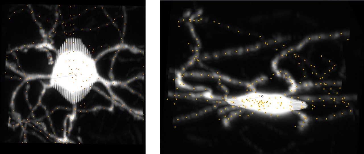
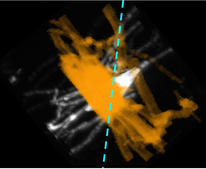
I did some more investigating to see how the labels were oriented. I tried swapping the different axes, it worked to some extent to orient but it did not solve the problem. It appears the labels are flipped along y=x, the following image is of the original labels rotated to depict a line of symmetry:
The latter is a more detailed image at different angles. The "additive" color filter is also used so the original image can be more visible underneath. The center image has 4 red dots to act as visual landmarks to show that this is indeed flipped. The cyan lines are the "plane of symmetry" that is observed.
The current version of the script is uploaded to this folder on the /frederick branch.
Steps:
-
Save the data as a
.tiffile. -
Run the line
runVaa3dPlugin(inFile=img_name, pluginName="Vaa3D_Neuron2", funcName="app2")to perform APP2, whereimg_nameis the name of the.tiffile. -
This function will automatically save a
.swcfile in the same folder that the original input image file is located in. Check there for output. -
I wrote a
.swcunpacker to read in the output and convert it to an Nx3numpyarray, where each row corresponds to anx,y,zof an output label. Napari can use this numpy array format to plot the labels, and I believe the coordinate list is a consistent format that can be used for other algorithms. -
I then plotted these labels in napari, overlaid on top of the original image:
We can see that for some reason, the labels appear to be rotated 90 degrees, or flipped along an axis. I'm not certain why this is the case, perhaps something went wrong with the .tif file saving, or an axis got flipped when generating the .swc file, I'm not sure. I will continue to debug this.
Running the line io.imsave(fname,img) with a fname that ends with ".tif" will save the image data array img as a .tif. file.
Vaa3D is an application built in C++ that can perform neuron tracing and segmentation on input image files. However, since we are downloading brains from an Amazon S3 instance, using the application locally proves to be a challenge. As such, I am resorting to using a Python Wrapper for Vaa3D so that we can run the plugin via a Python script.
- Download the Windows64 release version of Vaa3D v3.447
- Clone the pyVaa3D plugin repository
- Activate the Brainlit
condaenvironment,cdinto the pyVaa3D directory, andpip install -e . - Note that the original instructions are here
-
Import the method
from pyVaa3d.vaa3dWrapper import runVaa3dPlugin -
The
runVaa3dPluginmethod takes in aninfilename, the name of the specific Vaa3D plugin to run, and the specific function within the plugin. So far therunVaa3dPluginmethod appears to the following input types (list ongoing):.tiffiles,.swcfiles -
When importing this function, the terminal will prompt the user to enter the path to the executable
start_vaa3d.sh. Note that on Windows, the file is actuallyvaa3d_msvc.exe, located inside theC:Users\...\Vaa3D_V3.447_Windows_MSVC_64bit\directory. -
If it loads correctly, the Python terminal should look something like this:
Note that the highlighted portion is a user input.
-
The following line transforms the label outputs into a format that can be plotted using napari:
labels_plot = np.transpose(np.nonzero(labels))
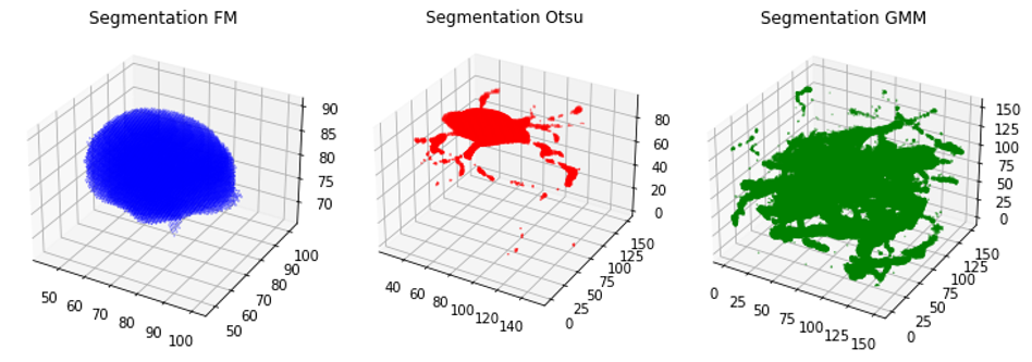
Otsu Segmentation:
FMM Segmentation:
GMM Segmentation:
We can see that the Otsu segmentation creates a very accurate representation of the original neuron but is perhaps an underestimate. FM is an extreme underestimate and only captures the cell body, while GMM captures too much of the random noise in the image.
We can roughly see how each of the segmentations look, but it's difficult to assess the performance without the original image as a reference.
Did some investigative work, I was able to run some of the segmentation algorithms in the adaptive_thresh.py file. Here are the labeling results:
FM seg foreground sum:  21209
FM seg total labels:  3442951
Otsu seg foreground sum:  28690
Otsu seg total labels:  3442951
GMM seg foreground sum:  283319
GMM seg total labels:  3442951
We can see that the labels returned are of the size 151 x 151 x 151, which is the volume of the sample image that we ran the demo on. At each index, it is either a 0 or a 1, which is either background or foreground.
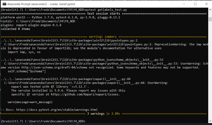
It follows that the labels returned by a segmentation algorithm should always span the volume of the input image. As such, I wrote a unit test to check for the length of the label vector returned. The output is seen below:
The test passed however there are a few warnings. These are related to module versions being out-of-date or possibly deprecated, but the code still functions. This may be a result of using a Python 3.7 environment instead of 3.8. The Napari warning might be easily solvable, will look into it later.
